| 2.4 |
Application of Differentiation |
|
| |
 |
| |
| Gradient of Tangent to a Curve at Different Points |
- The gradient changes at different points on a curve.
- The gradient function \(f'(x)\) is used to determine the gradient of tangent to the curve at any point on the function graph \(f(x)\).
- For example, for the function \(f(x)=x^2\):
| Value of \(x\) |
Gradient Function \(f'(x)=2x\) |
| \(-2\) |
\(-4\) |
| \(-1\) |
\(-2\) |
| \(0\) |
\(0\) |
| \(1\) |
\(2\) |
| \(2\) |
\(4\) |
|
|
| |
| The Equation of Tangent and Normal to a Curve at a Point |
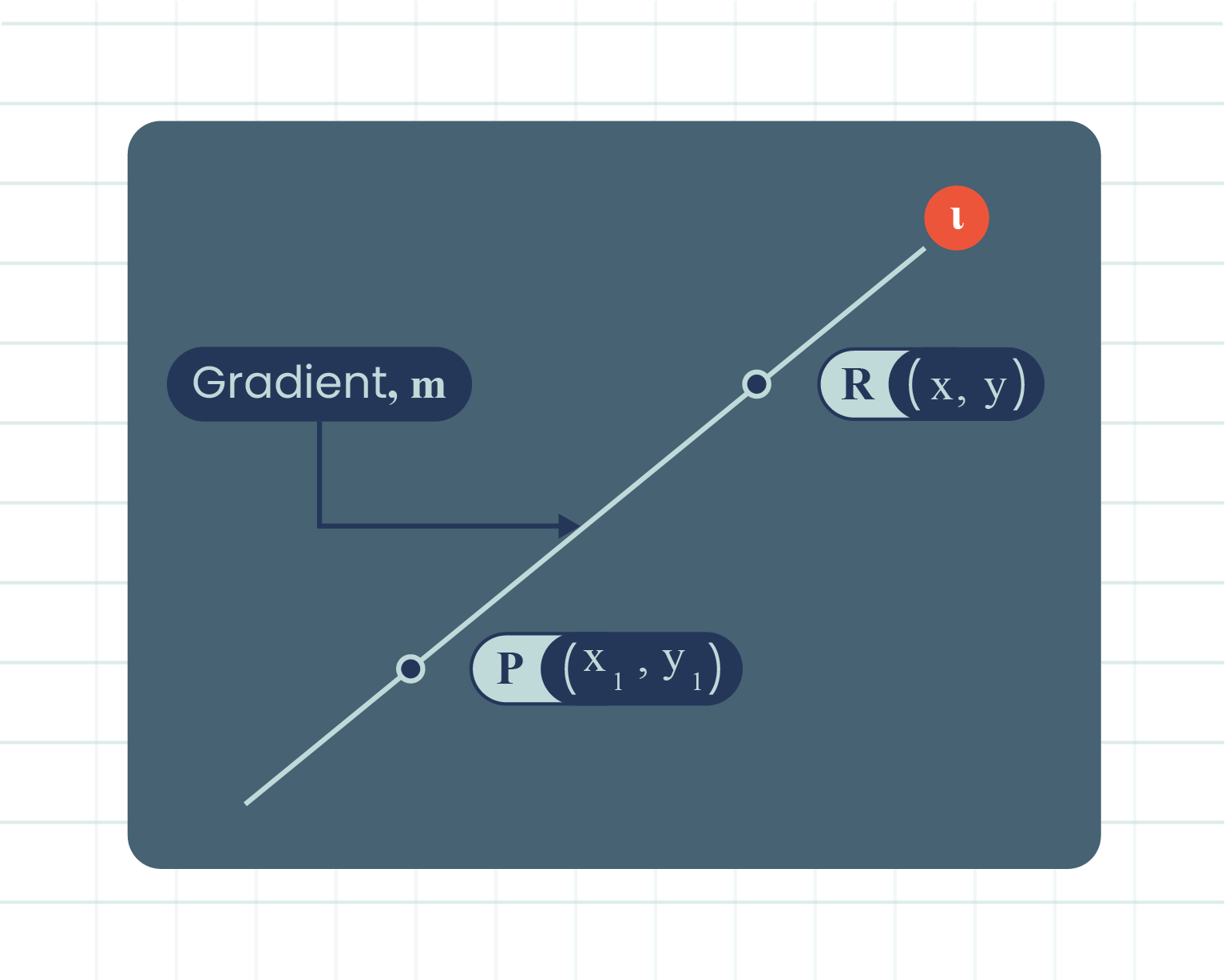
| Figure of Gradient of Tangent |
|
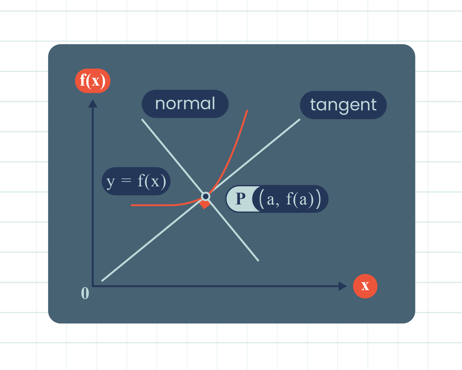
| Figure of Tangent and Normal |
|
- Based on the above diagram, the formula for the equation of straight line \(l\) with gradient \(m\) that passes through point \(P(x_1, y_1)\) can be written as:
\(y-y_1=m(x-x_1)\)
- The equation of the tangent is:
\(y-f(a)=f'(a)(x-a)\)
-
The line which is perpendicular to the tangent is the normal to the curve \(y=f(x)\) at point \(P(a,f(a))\).
-
If the gradient of the tangent, \(f'(a)\) exists and is non-zero, the gradient of the normal based on the relation of \(m_1m_2=-1\) is:
\(-\dfrac{1}{f'(a)}\)
- The equation of the normal is:
\(y-f(a)=-\dfrac{1}{f'(a)}(x-a)\)
|
|
| |
| Turning Points and Their Nature |
|
|
|
| |
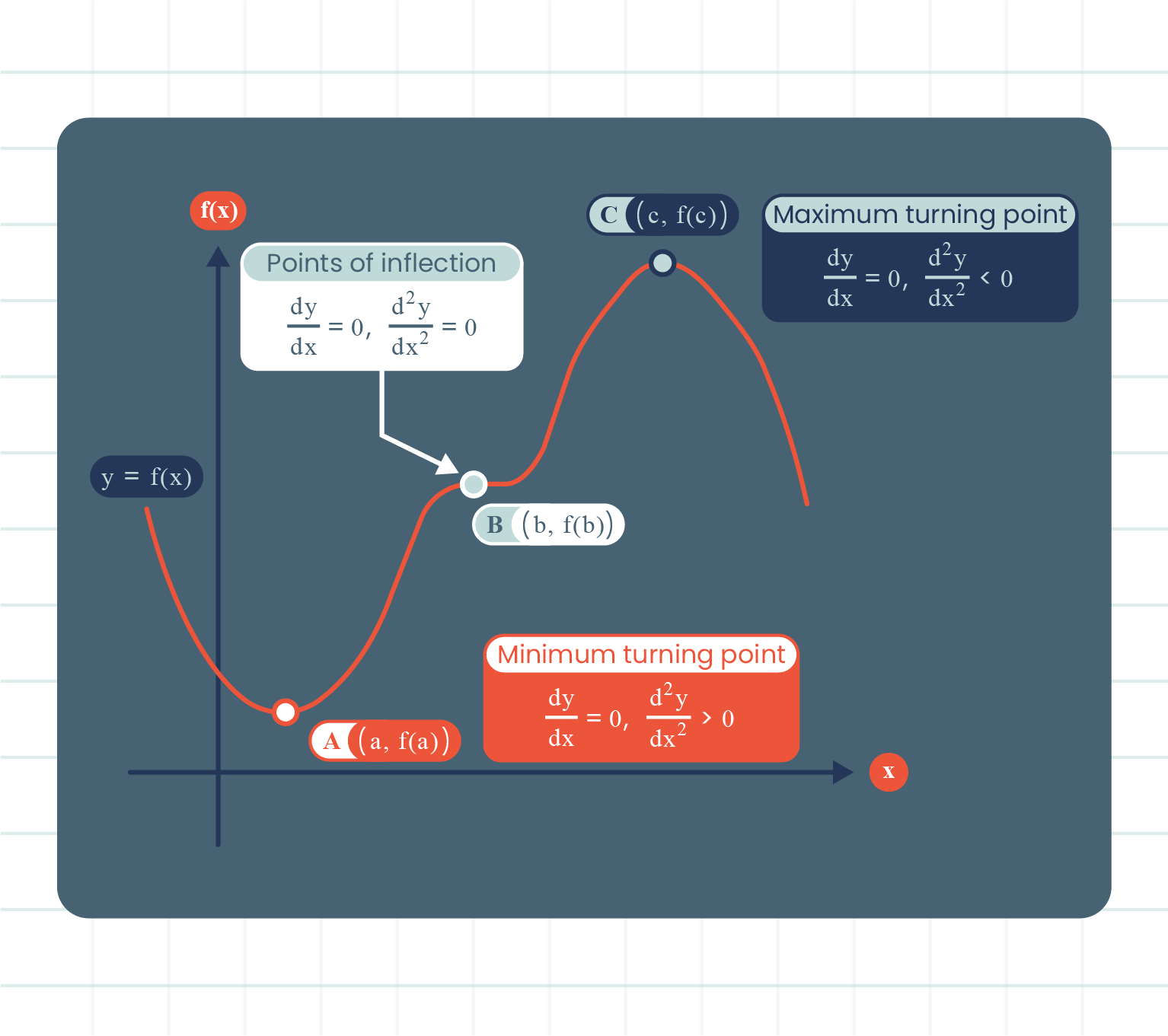
| \(3\) Types of Stationary Points |
- Turning points.
- When \(x\) increases through \(x=c\), the value of \(\dfrac{dy}{dx}\) changes sign from positive to negative.
|
- Turning points.
- When \(x\) increases through \(x=a\), the value of \(\dfrac{dy}{dx}\) changes sign from negative to positive.
|
- This stationary point which is not a maximum or a minimum point.
- A point on the curve at which the curvature of the graph changes.
- When \(x\) increases through \(x=b\), the value of \(\dfrac{dy}{dx}\) does not change in sign.
|
|
| |
| Conditions of Turning Points |
|
A turning point on a curve \(y=f(x)\) is a maximum point when \(\dfrac{dy}{dx}=0\) and \(\dfrac{d^2y}{dx^2} \lt 0\).
|
|
A turning point on a curve \(y=f(x)\) is a minimum point when \(\dfrac{dy}{dx}=0\) and \(\dfrac{d^2y}{dx^2} \gt 0\).
|
|
| |
| Change of \(y\) and \(x\) over time, \(t\) |
|
By applying the chain rule concept, if two variables, \(y\) and \(x\) change with time, \(t\) and are related by the equation \(y=f(x)\), then the rates of change \(\dfrac{dy}{dt}\) and \(\dfrac{dx}{dt}\) can be related by:
\(\dfrac{dy}{dt}=\dfrac{dy}{dx}\times \dfrac{dx}{dt}\)
|
|
| |
| Determining Small Changes and Approximations of Certain Quantities |
- If \(y=f(x)\) and the small change in \(x\), that is \(\delta x\) causes a small change in \(y\), \(\delta y\), then:
\(\delta y\approx\dfrac{dy}{dx} \times \delta x\)
- Since \(f(x+\delta x)=y+\delta y\) and \(\delta y\approx\dfrac{dy}{dx} \times \delta x\), then:
\(f(x+\delta x)=y+\dfrac{dy}{dx}\delta x\) or \(f(x+\delta x)=f(x)+\dfrac{dy}{dx}\delta x\)
- If \(x\) changes from \(x\) to \(x+\delta x\), then:
- The percentage change in \(x=\dfrac{\delta x}{x}\times 100\%\)
- The percentage change in \(y=\dfrac{\delta y}{y}\times 100\%\)
|
|
| |
| Example \(1\) |
|
Find the equation of the tangent and normal to the curve \(f(x)=x^3-2x^2+5\) at point \(P(2,5)\).
|
|
Given,
\(f(x)=x^3-2x^2+5\).
So,
\(f'(x)=3x^2-4x\).
At point \(P(2,5)\),
Gradient of the tangent:
\(\begin{aligned} f'(2)&=3(2)^2-4(2) \\ &=3(4)-8 \\ &=4. \end{aligned}\)
Equation of the tangent:
\(\begin{aligned} y-5&=4(x-2) \\ y-5&=4x-8 \\ y&=4x-8+5 \\ y&=4x-3. \end{aligned}\)
Gradient of the normal at point \(P(2,5)\):
\(\begin{aligned} m_Tm_N&=-1 \\ (4)m_N&=-1 \\ m_N&=-\dfrac{1}{4}. \end{aligned}\)
Equation of the normal:
\(\begin{aligned} y-5&=-\dfrac{1}{4}(x-2) \\ y-5&=-\dfrac{1}{4}x+\dfrac{1}{2} \\ y&=-\dfrac{1}{4}x+\dfrac{1}{2}+5 \\ y&=-\dfrac{1}{4}x+\dfrac{11}{2}. \end{aligned}\)
|
|
| |
| Example \(2\) |
|
Given \(y=x^3\), find
(a) the approximate change in \(y\) when \(x\) increases from \(4\) to \(4.05\),
(b) the approximate change in \(x\) when \(y\) decreases from \(8\) to \(7.97\).
|
|
(a)
\(y=x^3\),
\(\dfrac{dy}{dx}=3x^2\).
When \(x=4\),
\(\begin{aligned} \delta x&=4.05-4 \\ &=0.05 \\\\ \dfrac{dy}{dx}&=3(4)^2 \\ &=48 \\\\ \delta y &\approx \dfrac{dy}{dx}\times \delta x \\ &=48 \times 0.05 \\ \delta y &=2.4. \end{aligned}\)
Therefore, the approximate change in \(y\), \(\delta y\) is \(2.4\).
\(\delta y \gt 0\) means there is a small increase in \(y\) of \(2.4\).
(b)
When \(y=8\),
\(\begin{aligned} x^3&=8 \\ x&=2 \\\\ \delta y&=7.97-8 \\ &=-0.03 \\\\ \dfrac{dy}{dx}&=3(2)^2 \\ &=12 \\\\ \delta y &\approx \dfrac{dy}{dx} \times \delta x \\ -0.03&=12\times\delta x \\ \delta x&=\dfrac{-0.03}{12} \\ \delta x&=-0.0025. \end{aligned}\)
Therefore, the approximate change in \(x\), \(\delta x\) is \(-0.0025\).
\(\delta x \lt 0\) means there is a small decrease in \(x\) of \(0.0025\).
|
|
| |