|
|
| |
 |
| |
| Normal Distribution Function Graph |
|

|
| Features of a Normal Distribution Function Graph |
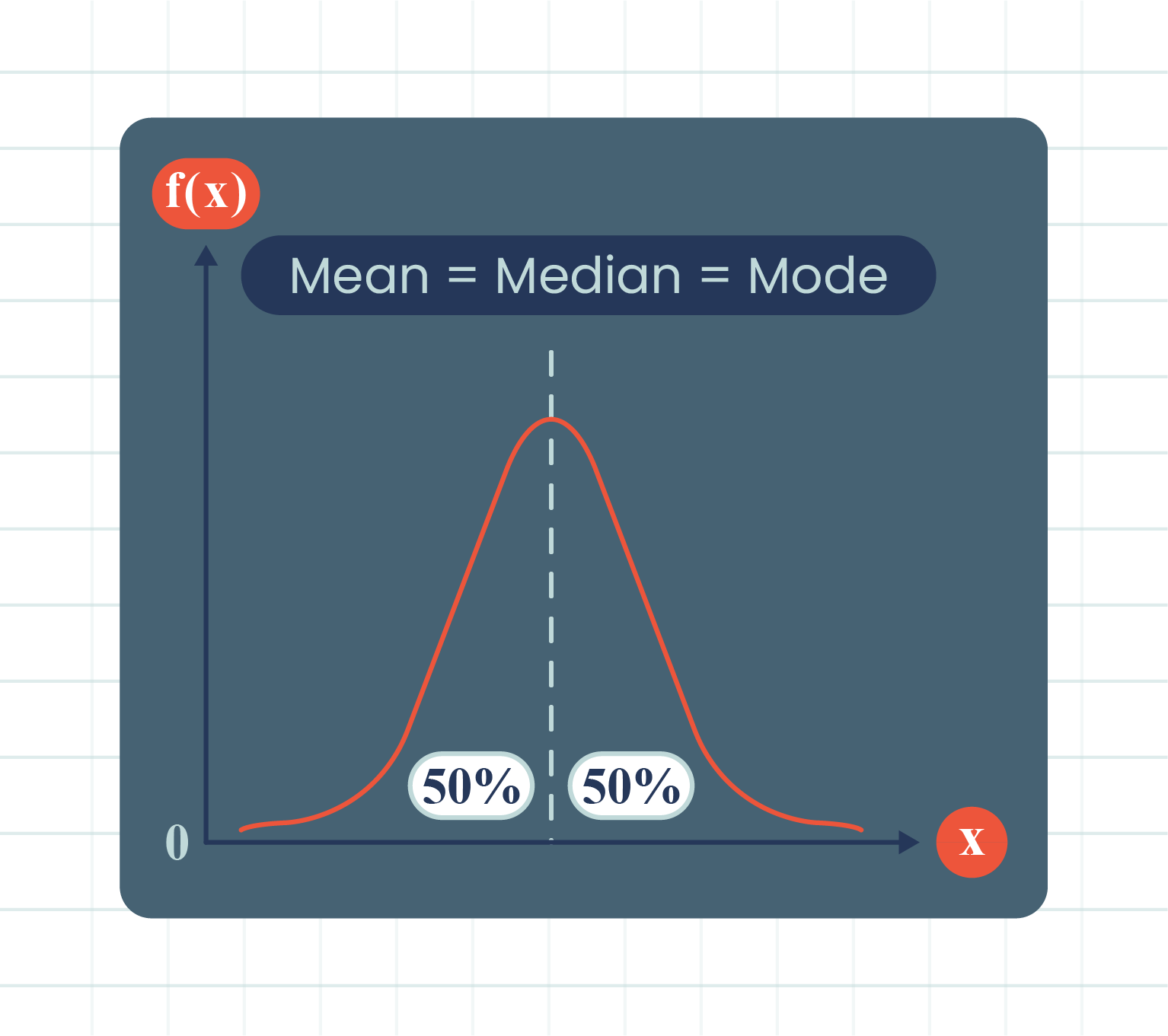
- The curve is bell-shaped and is symmetrical about a vertical line that passes through the mean, \(\mu\).
- The curve has a maximum value at the axis of symmetry, \(X=\mu\).
- The mean, \(\mu\) divides the region under the graph into two equal parts.
- Both ends of the curve extend indefinitely without touching the \(x\)-axis.
- The total area under the graph is equal to the total probability of all outcomes, that is, \(1\) unit\(^2\).
|
|
| |
| Notation Used for a Continuous Random Variable \(X\) Which has a Normal Distribution |
| \(X\sim N(\mu, \sigma^2)\) |
|
| |
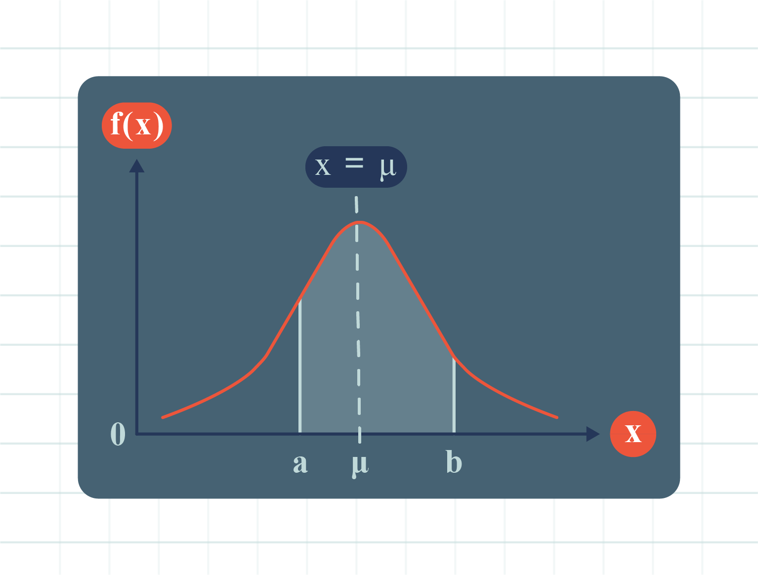
| The Area Under the Graph for \(X\) from \(a\) to \(b\) |
|

|
| Probability of \(X\) Occuring for the Value of \(X\) from \(a\) to \(b\) |
\(P(a \lt X \lt b)=P(a \leq X \leq b)\)
|
|
| |
| Random Variation and the Law of Large Numbers |
|
The larger the sample size, the smaller the random variation. So, the estimated value of a parameter becomes more consistent.
|
|
The larger the size of the sample, the value of the experimental mean gets closer to the theoretical mean value of the population.
|
|
| |
| Standard Normal Distribution |
- Standard normal distribution is defined as a normal distribution whose mean and standard deviation are \(0\) and \(1\) respectively.
- A continuous random variable \(X \sim N(\mu , \sigma^2)\) with mean \(\mu\) and standard deviation \(\sigma\) can be standardised by changing it to another continuous random variable \(Z\) whose mean is \(0\) and standard deviation is \(1\) by using the following formula:
\(Z=\dfrac{X-\mu}{\sigma}\), where \(Z\sim N(0,1)\)
|
|
| |
| Percentage of Data Distribution for Each Standard Normal Distribution |
- \(68\%\) of the data lies within the standard deviation \(\pm 1\) from the mean.
- \(95\%\) of the data lies within the standard deviation \(\pm 2\) from the mean.
- \(99.8\%\) of the data lies within the standard deviation \(\pm 3\) from the mean.
|
|
| |
| Probability of an Event for Normal Distribution |
|
To find the probability of a continuous random variable \(X\) that occurs between \(a\) and \(b\), we write it as \(P(a \lt X \lt b)\). Then, the way to convert this probability of the event to a standard normal distribution with a continuous random variable \(Z\) is as follows:
\(\begin{aligned} P(a\lt X \lt b)&=P\left( \dfrac{a-\mu}{\sigma} \lt \dfrac{X-\mu}{\sigma} \lt \dfrac{b-\mu}{\sigma} \right) \\ &=P \left( \dfrac{a-\mu}{\sigma} \lt Z \lt \dfrac{b-\mu}{\sigma} \right) \end{aligned}\)
|
|
| |
| Example \(1\) |
|

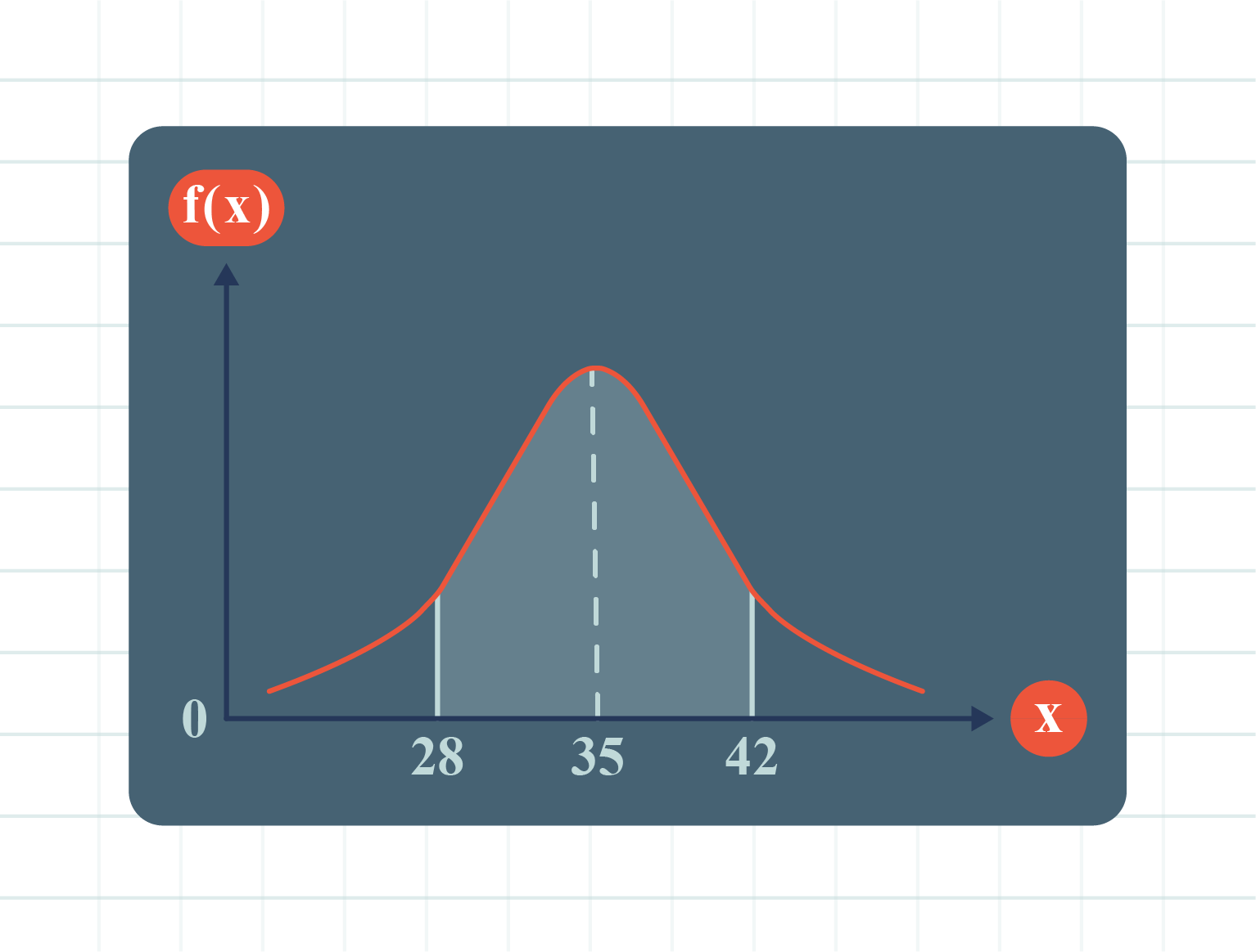
The diagram above shows a normal distribution function graph which is symmetrical at \(X=35\).
| (a) |
State the mean value, \(\mu\). |
| (b) |
Express the shaded region in probability notation. |
| (c) |
If the probability of the shaded region is \(0.64\), find \(P(X\text{ < }28)\). |
|
| (a) |
\(\mu=35\). |
| |
|
| (b) |
\(P(28\text{ < }X\text{ < }42)\). |
| |
|
| (c) |
Since the graph is symmetrical at \(X=35\) and \(X=28\) and \(X=42\) are both \(7\) units respectively to the left and right of the mean. Then, |
| |
\(\begin{aligned} P(X\text{ < }28)&=P(X\text{ > }42)\\\\ &=\dfrac{1-0.64}{2}\\\\ &=0.18. \end{aligned}\) |
|
|
| |
| Example \(2\) |
| (a) |
A continuous random variable \(X\) is normally distributed with mean \(30\) and a standard deviation of \(8\). |
| |
Find the \(z\)-score if \(X=42\). |
| |
|
| (b) |
The heights of buildings in Kampung Pekan are normally distributed with a mean of \(23\) m and a variance of \(25\) m\(^2\), find the height of the building if the standard score is \(0.213\). |
|
| (a) |
Given \(X=42\), \(\mu=30\) and \(\sigma=8\). |
| |
\(\begin{aligned} Z &= \dfrac{X-\mu}{\sigma}\\\\ &=\dfrac{42-30}{8}\\\\ &=1.5 .\end{aligned}\) |
| |
|
| (b) |
Given \(\mu=23\), \(\sigma^2=25\) and \(z\)-score\(=0.213\). |
| |
Then, |
| |
\(\begin{aligned} \sigma&=\sqrt{25} \\ &=5. \end{aligned}\) |
| |
Therefore, |
| |
\(\begin{aligned} Z &= \dfrac{X-\mu}{\sigma}\\\\ 0.213&=\dfrac{X-23}{5}\\\\ 1.065&=X-23\\\\ X&=24.065\text{ m}. \end{aligned}\) |
|
|
| |
| Example \(3\) |
|
The lengths of a type of screw produced by a factory can be considered as normally distributed with a mean of \(10.6\) cm and a standard deviation of \(3.2\) cm.
Represent the probability that a screw randomly chosen from the factory has a length between \(8.4\) cm and \(13.2\) cm where \(Z\) is a standard continuous random variable.
|
|
Let \(X\) represent the length of the screw produced by the factory.
Given \(\mu=10.6\) and \(\sigma=3.2\).
\(\begin{aligned} &P(\text{Length of screw is between }8.4\text{ cm and }13.2\text{ cm})\\\\ &= P(8.4 \text{ < } X \text{ < } 13.2)\\\\ &=P\begin{pmatrix}\dfrac{8.4-10.6}{3.2} \text{ < } \dfrac{X-\mu}{\sigma} \text{ < } \dfrac{13.2-10.6}{3.2}\end{pmatrix}\\\\ &=P(-0.6875 \text{ < } Z\text{ < } 0.8125) .\end{aligned}\)
|
|
| |