|
|
| |
 |
| |
| Two Types of Random Variables |
| Discrete Random Variable |
Continuous Random Variable |
| Random variables that have countable numbers of values, usually taking values like zero and positive integers. |
Random variables that are not integers but take values that lie in an interval. |
|
|
| |
| Discrete Random Variable |
|
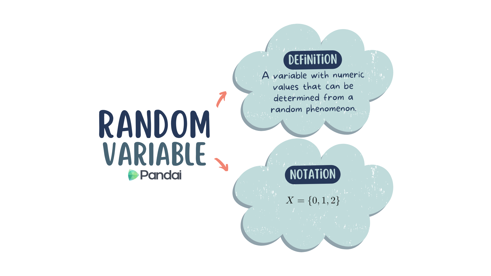
If \(X\) represents a discrete random variable, hence the possible outcomes can be written in set notation:
\(X = \lbrace r : r = 0, 1, 2, 3\rbrace\)
|
|
| |
| Continuous Random Variable |
|
If \(Y\) represents a continuous random variable, hence the possible outcomes can be written as:
\(Y = \lbrace y : y\) is the pupil's height in cm, \(a \leq y \leq b \rbrace\)
|
|
| |
| Probability Distribution for Discrete Random Variables |
| If \(X\) is a discrete random variable with the values \(r_1\), \(r_2\), \(r_3\), \(...\), \(r_n\) and their respective probabilities are \(P(X=r_1)\), \(P(X=r_2)\), \(P(X=r_3)\), \(...\), \(P(X=r_n)\), then \(\sum_{i=1}^{n} P(X=r_i)=1\), thus each \(P(X=r_i) \geq0\). |
|
| |
| Example |
|
\(70\%\) of Form \(5\) Dahlia pupils achieved a grade A in the final year examination for the Science subject. Two pupils were chosen at random from that class.
| (a) |
If \(X\) represents the number of pupils who did not get a grade A, construct a table to show all the possible values of \(X\) with their corresponding probabilities. |
| (b) |
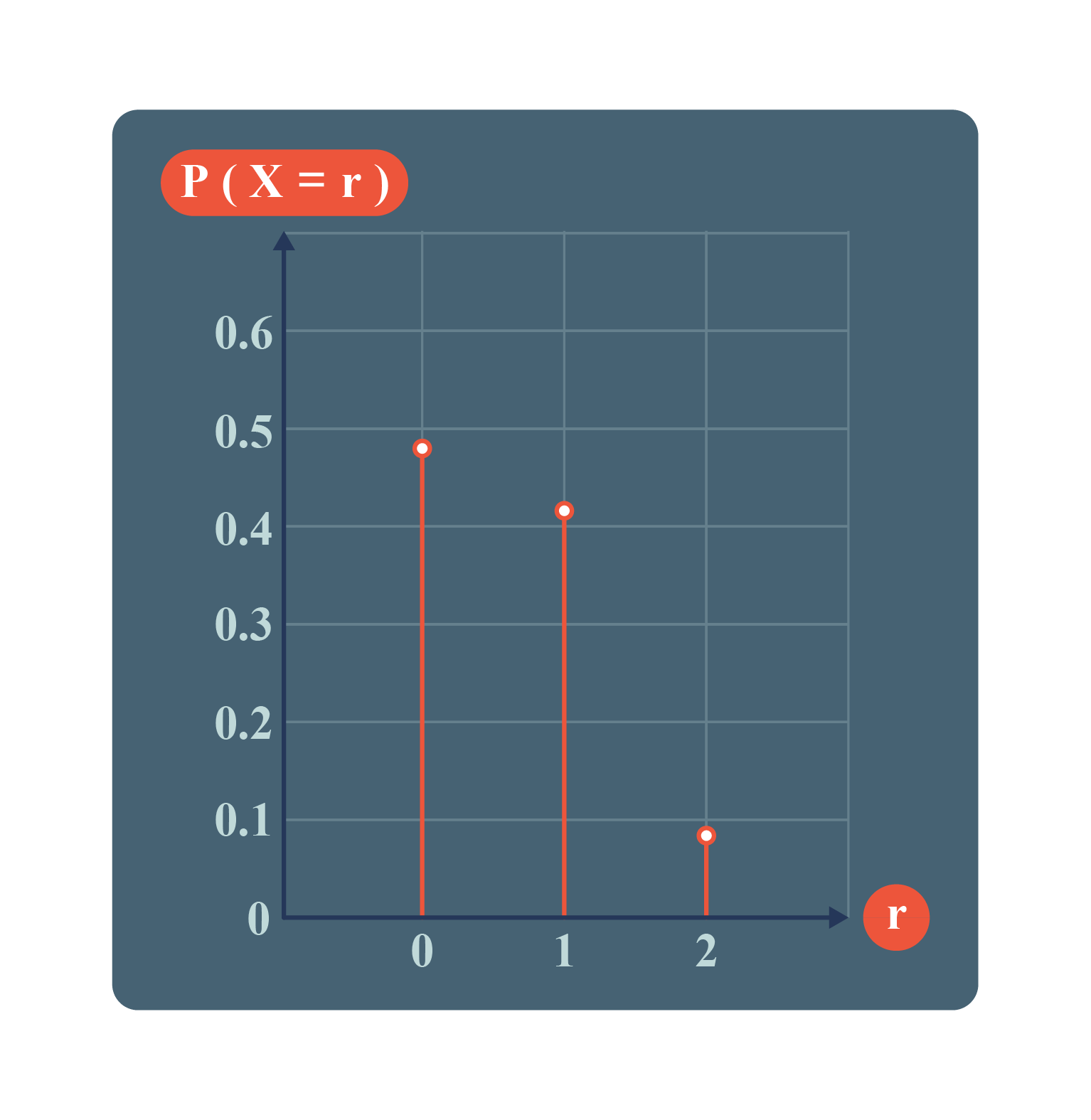
Next, draw a graph to show the probability distribution of \(X\). |
|
|
\(P (A : A \text{ is a pupil who did not achieve a grade A}) \\ = 1-\dfrac{70}{100}\\ = 0.3.\)
\(P (B : B \text{ is a pupil who achieved a grade A}) \\ = \dfrac{70}{100}\\ = 0.7.\)
Then, \(X = \{0, 1, 2\}\).
\(\begin{aligned} P(X = 0) &= P(B, B) \\ &= 0.7 × 0.7\\ &=0.49.\\\\ P(X = 1) &= P(A, B) + P(B, A)\\ &= (0.3 × 0.7) + (0.7 × 0.3)\\ &=0.42.\\\\ P(X = 2) &= P(A, A) \\ &= 0.3 × 0.3\\ &=0.09 .\end{aligned}\)
| \(X=r\) |
\(0\) |
\(1\) |
\(2\) |
| \(P(X=r)\) |
\(0.49\) |
\(0.42\) |
\(0.09\) |
|
|
|
|
| |